tags:
  - fundamentals
  - dataviz
  - deep_learning
  - interpretability
  - dimensionality_reduction
Latent spaces
https://digital-garden-betheve-ff4539b5328d87e722420cea05c7e2905bd94833.gitpages.huma-num.fr/lib/media/visualization-of-the-deepsdf-latent-space-using-t-sne.mp4# What is a latent space
Latent space is a lower-dimensional space into which high-dimensional data transforms. Projecting a vector or matrix into a latent space aims at capturing the data’s essential attributes or characteristics in fewer dimensions.
The simplest deep learning architecture using a latent space is that of the Autoencoders, which follows an encoder-decoder concept. The latent space is the lowest dimension layer, in other terms, the one with the least neurons.
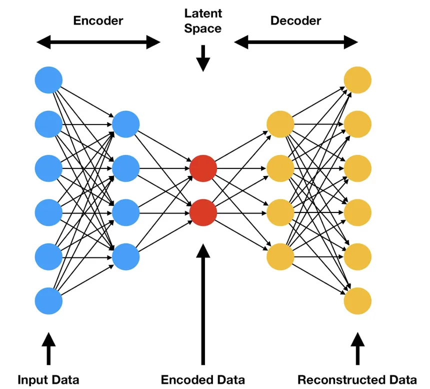
This Latent Space holds the embedded representation of the high-dimension input vectors into a vector space which holds these compressed representations, also known as vector embeddings.
To embed here means that the model learns to reduce the size of the data while maintaining the most information possible, similar to compression.
In other words, the back and forth encoding-decoding training converges towards a summarized version of the input data, which is no longer directly human-readable, but where the similar data is close to each other in this space, and dissimilar data is further.
For a more formal definition :
A latent space, also known as a latent feature space or embedding space, is an embedding of a set of items within a manifold in which items resembling each other are positioned closer to one another. Position within the latent space can be viewed as being defined by a set of latent variables that emerge from the resemblances from the objects.
In short, a latent space is a more compact representation of the data.
The idea that high-dimensionality data can be compressed while retaining most of its information and why machine learning works so well is called The Manifold Hypothesis
What problem does it solve
Visualisation tools
Visual Resources :
Latent Space Visualisation: PCA, t-SNE, UMAP | Deep Learning Animated
Variational Autoencoder (VAE) Latent Space Visualization
Google : A.I. Experiments: Visualizing High-Dimensional Space
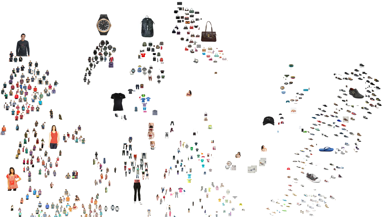
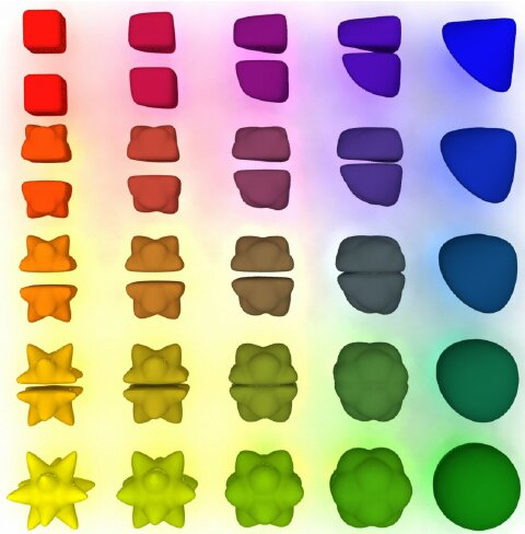
On the fashion MNIST Dataset, we can visualize the latent space to understand some relationships between data, where similar data is clustered together. From this we can deduce some transformation vectors that go from flip-flop images to formal shoes images.
What can we do with it ?
Synthetic Data generation
Before Generative Adversarial Networks or Diffusion Models, one of the ways we can generate synthetic data is by doing inverse transforms projections of latent space vectors.
In other words, we can reverse-engineer the input by using inverse transforms to generate new data like such :
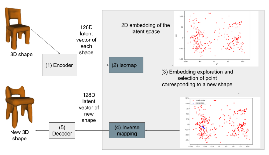
image source
For example, for image generation, we would take a sample point from the final latent space, and use the decoder part of the network to generate a totally new image that is within the bounds of the latent space. In other words, if we trained a model on cats and dogs pictures, we can only generate cats and dogs pictures, or something in-between a cat and a dog.
Computing the in-between of two vectors or points in a given space, is called interpolation, therefore, in latent space, we have latent interpolation.
Latent space interpolation
An interpolation in the latent space between multiple vectors can yield the intermediate states to go from one state to another.
This is what is illustrated at the beginning of this article with this video :
By navigating the latent space, we can go from the chair cluster to the table and couch clusters to get how to morph one thing into another.
There are many ways to do that, that achieve different goals, depending on how you compute the distance ; in other words, which metric is used.
Something that achieves similar results but with a different approach :
Optimal Transport is a sub-field of Machine Learning that can compute intermediary states between statistical distributions.
It can also be applied to images or any signals if they are considered to be a sample from a statistical distribution, as is assumed in most cases. It does not rely on latent spaces though.
It uses Wasserstein Distance instead of Euclidian distance to compute the intermediate states, also called barycenters. This is illustrated in the following figure.
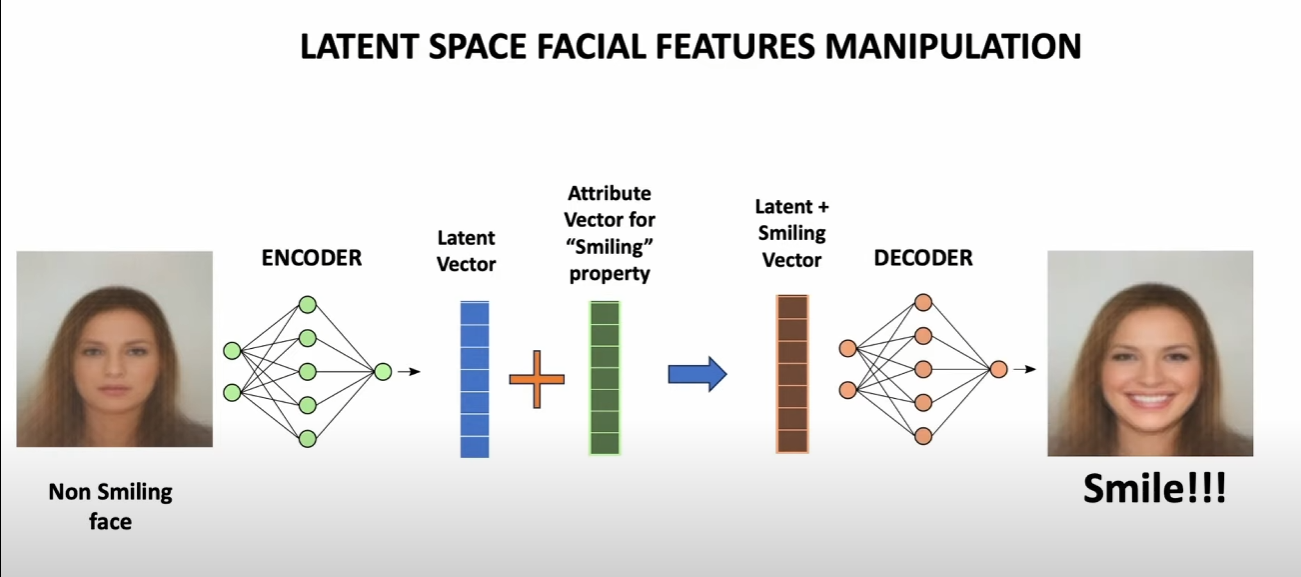
Latent space arithmetics
Once our latent space is established, we can reverse-engineer the input data to produce variations of the input given a feature.
For example, here, we take a non-smiling face image as input, and apply the "smiling" transformation to the encoded input vector corresponding to the input image, and we can reconstruct a smiling face image from the baseline !
We can go further and chain those operations to get specific results :